The Eigenvalue Problem That Changed How I Saw Math

I used to hate math. Well, maybe hate isn’t the best word, but I wouldn’t say I necessarily enjoyed my math classes in High School. Indifferent, I guess, is a good descriptor of my past relationship with math. That is, until my second semester of college.

This semester (Spring 2025) I was in MA 26200 - Linear Algebra and Differential Equations. I was apprehensive about entering this new realm of math – until I discovered the YouTube channel 3 Blue 1 Brown and their Intro to Linear Algebra series. After watching a couple of videos, that indifference began to transform into slight curiosity, which quickly snowballed into fascination. Their complex yet beautiful visuals explained how Linear Algebra worked on a quantitative and qualitative level, and demonstrated how abstract concepts could have very concrete meanings behind them. The previously uninteresting world of math began to seem inviting, and I started to become curious as to what else lay inside. After my MA 262 lecture on Eigenvectors and Eigenvalues, I immediately went and watched 3b1b’s video on the topic. And to my surprise (and perhaps even delight), he ended the video with this challenge problem:

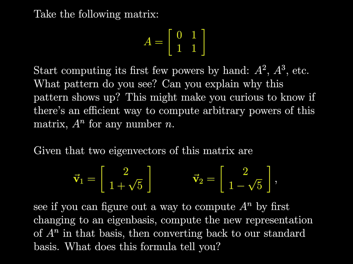
Instinctively, I almost rejected the idea of doing a math problem what I wasn’t required to do. But after reading the problem a few more times, my curiosity took over and I decided to give it a shot. How hard could it be? (spoiler alert: actually kinda hard but in a good way)

The problem starts by telling you to compute the first few powers of the matrix \(\mathbf{A} = \begin{bmatrix}0 & 1\\1 & 1\end{bmatrix}\) by hand, yielding the following results:

\(\) \(\qquad \mathbf{A} ^ 1 = \begin{bmatrix}0 & 1\\1 & 1\end{bmatrix} \quad \mathbf{A} ^ 2 = \begin{bmatrix}1 & 1\\1 & 2\end{bmatrix} \quad \mathbf{A} ^ 3 = \begin{bmatrix}1 & 2\\2 & 3\end{bmatrix} \quad \mathbf{A} ^ 4 = \begin{bmatrix}2 & 3\\3 & 5\end{bmatrix} \quad \mathbf{A} ^ 5 = \begin{bmatrix}3 & 5\\5 & 8\end{bmatrix} \quad \mathbf{A} ^ 6 = \begin{bmatrix}5 & 8\\8 & 13\end{bmatrix} \quad\)

In order to develop a formula for \(\mathbf{A}^n\), we first have to ‘diagonalize’ it – that is, convert it to a matrix where all values outside of the diagonal are zero. That’s because the nth power of a diagonal matrix is the nth power of each term. For example: if \(\mathbf{A} = \begin{bmatrix}a & 0\\0 & b\end{bmatrix}\), then \(\mathbf{A}^n = \begin{bmatrix}a^n & 0\\0 & b^n\end{bmatrix}\)

Now, in order to convert our original transformation matrix \(\mathbf{A}\) into a diagonal matrix, we can take advantage of a property of diagonal matrices: they are scalar transformations and have no rotational effect when applied (multiplied) to a vector. Now, this property should be setting off alarm bells for any linear algebra student: it’s very similar to the definition of an eigenvector! Thus, if we can express \(\mathbf{A}\) in terms of its eigenvectors, we will have a diagonal matrix, which we can then easily raise to the power of n.

There’s just one problem: how can we express a matrix in terms of another set of vectors? Well, it’s conceptually pretty simple: right now, we’re used to expressing all 2D vectors and matrices in terms of our standard basis vectors \(\hat{\imath} = \begin{bmatrix}1 \\ 0\end{bmatrix}\) and \(\hat{\jmath} = \begin{bmatrix}0 \\ 1\end{bmatrix}\). What this means mathematically is that a vector \(\begin{bmatrix}a \\ b\end{bmatrix}\) can represented as \(a\cdot\hat{\imath} + b\cdot\hat{\jmath}\). By this logic, we could utilize any set of vectors as our basis vectors, and express any vector or matrix in terms of our new basis vectors. And here’s the important piece: if we choose the eigenvectors of a matrix as the basis vectors, then said matrix expressed in terms of that new basis will be a diagonal matrix - a process known as eigendecomposition.

That may be a lot of information at once, but take a second to conceptualize it, and recall the definition of an eigenvector: \(\vec{\mathbf{v}}\mathbf{M} = \lambda\mathbf{M}\). It’s as if we’re transforming the entire coordinate space so the basis vectors fall on the eigenvectors – actually, that’s exactly what we’re doing. If you want to see this visualized, check out 3B1B.

But how do you express a matrix in terms of a new set of basis vectors? This operation is fittingly called a Change of Basis operation; to demonstrate it, let’s first imagine we have a vector \(\vec{\mathbf{v}}_b\) in terms of a different basis and we want to apply a transformation \(A\) from our standard basis to it. Also, we know the set of basis vectors for \(\vec{\mathbf{v}}_b\), which can be expressed in our standard basis as \(\vec{b_x}\hat{\imath} + \vec{b_y}\hat{\jmath}\). So in order to apply \(\mathbf{A}\) to \(\vec{\mathbf{v}}_b\), we first have to express \(\vec{\mathbf{v}}_b\) in terms of our standard \(\hat{\imath}\) and \(\hat{\jmath}\) basis. We can do this by applying the transformation \(\mathbf{B}\vec{\mathbf{v}}_b\), where the column space of \(\mathbf{B}\) is the basis vectors of \(\vec{\mathbf{v}}_b\), i.e., \(\mathbf{B} = \begin{bmatrix}\vec{b_x}&\vec{b_y}\end{bmatrix}\). This operation expresses \(\vec{\mathbf{v}}_b\) in terms of our standard \(\hat{\imath}\) and \(\hat{\jmath}\) basis. I could go in depth as to why this is true, but I’ll leave that as an excercise for the reader :). This matrix \(\mathbf{B}\), where the column space is some other set of basis vectors, is called a Change of Basis matrix.

Now that we have \(\vec{\mathbf{v}}_b\) in terms of \(\hat{\imath}\) and \(\hat{\jmath}\), we can apply our transformation \(\mathbf{A}\), leaving us with \(\mathbf{AB\vec{v}}_b\). What we have so far is the vector \(\vec{\mathbf{v}}_b\) converted to our standard basis using the change of basis matrix, then transformed using \(\mathbf{A}\). The final step is to convert it back to its original matrix, which is done by applying the inverse of the change of basis matrix, essentially just undoing the first change of basis transformation while retaining the transformation from \(\mathbf{A}\). This leaves us with the final equation \(\mathbf{B^{-1}AB\vec{v}}_b\). Thus, \(\mathbf{B}^{-1}\mathbf{AB}\) expresses the transformation \(\mathbf{A}\) in terms of the column space of \(\mathbf{B}\).

With that out of the way, we can now apply this to the original problem. Our goal is to express the transformation matrix \(\mathbf{A}\) in terms of the eigenvectors, so we can start by defining \(\mathbf{B}\) as follows:

\[\mathbf{B} = \begin{bmatrix}\vec{\mathbf{v}}_2&\vec{\mathbf{v}}_2\end{bmatrix},\quad\vec{\mathbf{v}}_1=\begin{bmatrix}2\\1+\sqrt{5}\end{bmatrix}\quad\vec{\mathbf{v}}_2=\begin{bmatrix}2\\1-\sqrt{5}\end{bmatrix},\quad\therefore\quad \mathbf{B} = \begin{bmatrix}2&2\\1+\sqrt{5}&1-\sqrt{5}\end{bmatrix}\]

Now before we go any further, this matrix can actually be simplified by dividing each term by two. Now \(\mathbf{B} = \begin{bmatrix}1&1\\\frac{1+\sqrt{5}}{2}&\frac{1-\sqrt{5}}{2}\end{bmatrix}\). Conveniently, the terms in the second row happen to be both of the eigenvalues of \(\mathbf{A}\), and we can substitute the values there for their symbols to reach our final form for \(\mathbf{B}\) and \(\mathbf{B}^{-1}\):

\[\mathbf{B}=\begin{bmatrix}1&1\\\lambda_1&\lambda_2\end{bmatrix}\quad\mathbf{B}^{-1}=\begin{bmatrix}-\lambda_2&1\\\lambda_1&-1\end{bmatrix}\dfrac{1}{\sqrt{5}}\]

Just a side note: if you don’t do these last two changes and try to solve, it will be very messy. I know this since I spent like two nights doing it this way.

Solving \(\mathbf{B}^{-1}\mathbf{AB}\) with our new values yields the following:\(\quad\mathbf{B}^{-1}\mathbf{AB} = \dfrac{1}{\sqrt{5}}\begin{bmatrix}-\lambda_2&1\\\lambda_1&-1\end{bmatrix} \begin{bmatrix}1&1\\\lambda_1&\lambda_2\end{bmatrix} \begin{bmatrix}0 & 1\\1 & 1\end{bmatrix}\)

Solving this yields the following diagonalized matrix:

\[\mathbf{B}^{-1}\mathbf{AB} = \begin{bmatrix}\lambda_1&0\\0&\lambda_2\end{bmatrix}\]

What a beautiful and convenient solution! Conceptually this checks out too – in the chosen eigenbasis, this transformation scales its eigenvectors by a factor of its eigenvalues. And now that its diagonalized, we can easily raise it to the nth power: \(\begin{bmatrix}\lambda_1^n&0\\0&\lambda_2^n\end{bmatrix}\)

But this matrix is still in terms of the eigenvalues. Now that we’ve applied the nth power to it, we need to convert it back to being in terms of our regular basis. Doing this is actually pretty easy – just use the same concept as before, but backwards. This yields the following equation,

\[\mathbf{A}^n = \mathbf{B}(\mathbf{B}^{-1}\mathbf{AB})^n\mathbf{B}^{-1} = \begin{bmatrix}1&1\\\lambda_1&\lambda_2\end{bmatrix} \begin{bmatrix}\lambda_1^n&0\\0&\lambda_2^n\end{bmatrix} \begin{bmatrix}-\lambda_2&1\\\lambda_1&-1\end{bmatrix}\dfrac{1}{\sqrt{5}}\]

which when solved yields

\[\begin{bmatrix}\lambda_1\lambda_2^n-\lambda_2\lambda_1^n & \lambda_1^n-\lambda_2^n \\\lambda_1\lambda_2^{n+1}-\lambda_2\lambda_1^{n+1} & \lambda_1^{n+1}-\lambda_2^{n+1}\end{bmatrix}\dfrac{1}{\sqrt{5}}\]

which can be simplified further to yield the final equation:

\[\mathbf{A}^n = \begin{bmatrix}\lambda_1^{n-1}-\lambda_2^{n-1} & \lambda_1^n-\lambda_2^n \\ \lambda_1^n-\lambda_2^n & \lambda_1^{n+1}-\lambda_2^{n+1}\end{bmatrix}\dfrac{1}{\sqrt{5}}, \quad\lambda_1 = \dfrac{1 + \sqrt{5}}{2}, \quad\lambda_2 = \dfrac{1 - \sqrt{5}}{2}\]

This formula successfully computes \(\mathbf{A}^n\) for all values of n! And interestingly enough, the equation for the top-right and bottom-left entries in the matrix is known as Binet’s Formula, which is more commonly written as

\[F_n = \frac{\varphi^n - \psi^n}{\sqrt{5}}, \quad\varphi = \dfrac{1 + \sqrt{5}}{2} = \lambda_1, \quad\psi = 1 - \overline{\varphi} = \lambda_2\]

Here, \(\varphi\) is a value known as the golden ratio; this value along with the Fibonacci pattern is found in many areas of mathematics as well as nature and design.

---

Solving this problem was not only a fun challenge but represents a fundamental shift in my view of mathematics as a whole. Finding this sudden beauty in abstraction was a new experience for me. Like I emphasized earlier, I used to view math as being an insignificant annoyance. But after being captivated by 3Blue1Brown’s content, I began to realize that math could be more than just an inconvenience. I can be interested by it and explore it further; it’s just up to me to allow myself to do that. In high school it was easy to dismiss math as “something for nerds,” but college showed me that exploring my interests is something I not only can do but am encouraged to do.

I’ve been fascinated by how math and physics collide to form engineering. That’s what engineering is fundamentally about, but it’s easy to lose that with the boring generic engineering jobs that so many people end up in. I truly hope that by embracing my interest in mathematics, I can find a fulfilling future within engineering.

Another thing I learned is that (most) professors are super nice! I stopped by the office hours of Professor Joseph (Kuan-Hua) Chen – the Purdue Math Department Assistant Head and creator of Chenflix (if you don’t know what this is just ask any Purdue student) – and he was super excited to help me on this problem. I was already mostly finished, but together we worked through it from scratch. We then talked a bit more about math, and a couple days later I went back to chat with him about my newfound interest in math. He gave me some book recommendations and invited me to return any time to talk. Having the genuine support of such an amazing professor has encouraged me to explore my own interests; I plan on continuing this by independent studying control systems this summer.

I hope you enjoyed reading about this journey! This is my first post here so sorry if it’s a bit wordy or unpolished, I hope to improve my writing and thought process by creating more posts here. Stay tuned for more! Peace.